Glossary

K8S：k8s is short for Kubernetes, which is an open-source container orchestration platform that provides automated deployment, scaling, and management of containerized applications. It can run on various cloud platforms, physical servers, and virtual machines, and supports multiple container runtimes, enabling high availability, load balancing, automatic scaling, and automatic repair, and other functions.

Graph Processing： Graph Processing is a computing model used to solve computational problems related to graph data structures. The graph computing model can be applied to solve many real-world problems, such as social network analysis, network traffic analysis, medical diagnosis, and more.

ISO-GQL：GQL is a standard query language for property graphs, which stands for "Graph Query Language", and is an ISO/IEC international standard database language. In addition to supporting the Gremlin query language, GeaFlow also supports GQL. This means that GeaFlow users can use the GQL language to query and analyze their graph data, thereby enhancing their graph data processing capabilities.

Cycle： The GeaFlow Scheduler is a core data structure in the scheduling model. A cycle is described as a basic unit that can be executed repeatedly, and it includes a description of input, intermediate calculations, data exchange, and output. It is generated by the vertex groups in the execution plan and supports nesting.

Event： The core data structure for the interaction between scheduling and computation at the Runtime layer is the Scheduler. The Scheduler constructs a state machine from a series of event sets and distributes it to workers for computation and execution. Some of these events are executable, meaning they have their own computational semantics, and the entire scheduling and computation process is executed asynchronously.

Graph Traversal : Graph Traversal refers to the process of traversing all nodes or some nodes in a graph data structure, visiting all nodes in a specific order, mainly using depth-first search (DFS) and breadth-first search (BFS). It is used to solve many problems, including finding the shortest path between two nodes, detecting cycles in a graph, and so on.

Graph State： GraphState is used to store the graph data or intermediate results of graph iteration calculations in Geaflow. It provides exactly-once semantics and the ability to reuse jobs at the job level. GraphState can be divided into two types: Static and Dynamic. Static GraphState views the entire graph as a complete entity, and all operations are performed on a complete graph. Dynamic GraphState assumes that the graph is dynamically changing and is composed of time slices, and all slices make up a complete graph, and all operations are performed on the slices.

Key State： KeyState is used to store intermediate results during the calculation process and is generally used for stream processing, such as recording intermediate aggregation results in KeyState when performing aggregation. Similar to GraphState, Geaflow regularly persists KeyState, so KeyState also provides exactly-once semantics. Depending on the data result, KeyState can be divided into KeyValueState, KeyListState, KeyMapState, and so on.

Graph View

Fundamental Conception

GraphView is the critical core data abstraction in Geaflow, representing a virtual view based on graph structure. It is an abstraction of graph physical storage, which can represent the storage and operation of graph data on multiple nodes. In Geaflow, GraphView is a first-class citizen, and all user operations on the graph are based on GraphView. For example, distributing point and edge streams as GraphView incremental point/edge data sets, generating snapshots for the current GraphView, and triggering calculations based on snapshot graphs or dynamic GraphViews.

Functional Description

GraphView has the following main functions:

• Graph manipulation：it can add or delete vertex and edge data, as well as perform queries and take snapshots based on a specific time slice.
• Graph storage: it can be stored in a graph database or other storage media (such as a file system, KV storage, wide-table storage, native graph, etc.).
• Graph partitioning: it also supports different graph partitioning methods.
• Graph computation: it can perform iterative traversal or computation on the graph.

Example Introduction

Define a GraphView for a social network that describes interpersonal relationships.

DSL Code

CREATE GRAPH social_network (
	Vertex person (
	  id int ID,
	  name varchar
	),
	Edge knows (
	  person1 int SOURCE ID,
	  person2 int DESTINATION ID,
	  weight int
	)
) WITH (
	storeType='rocksdb',
	shardCount = 128
);

HLA Code

//build graph view.
final String graphName = "social_network";
GraphViewDesc graphViewDesc = GraphViewBuilder
	.createGraphView(graphName)
	.withShardNum(128)
	.withBackend(BackendType.RocksDB)
    .withSchema(new GraphMetaType(IntegerType.INSTANCE, ValueVertex.class,
                String.class, ValueEdge.class, Integer.class))
	.build();

// bind the graphview with pipeline1
pipeline.withView(graphName, graphViewDesc);
pipeline.submit(new PipelineTask());

Stream Graph

Fundamental Conception

The term "Streaming Graph" refers to graph data that is stream-based, dynamic, and constantly changing. Within the context of GeaFlow, Streaming Graph also refers to the computing mode for streaming graphs, Which is designed for graphs that undergo streaming changes, and performs operations such as graph traversal, graph matching, and graph computation based on graph changes.

Based on the GeaFlow framework, it is easy to perform dynamic computation on streaming graphs. In GeaFlow, we have abstracted two core concepts: Dynamic Graph and Static Graph.

• Static Graph refers to a static graph, in which the nodes and edges are fixed at a certain point in time and do not change. Computation on Static Graph is based on the static structure of the entire graph, so conventional graph algorithms and processing can be used for computation.

• Dynamic Graph refers to a dynamic graph, where nodes and edges are constantly changing. When the status of a node or edge changes, Dynamic Graph updates the graph structure promptly and performs computation on the new graph structure. In Dynamic Graph, nodes and edges can have dynamic attributes, which can also change with the graph. Computation on Dynamic Graph is based on the real-time structure and attributes of the graph, so special algorithms and processing are required for computation.

GeaFlow provides various computation modes and algorithms based on Dynamic Graph and Static Graph to facilitate users' choices and usage based on different needs. At the same time, GeaFlow also supports custom algorithms and processing, so users can extend and optimize algorithms according to their own needs.

Functional Description

Streaming Graph mainly has the following features:

• Supports streaming processing of node and edge data, but the overall graph is static.
• Supports continuous updates and queries of the graph structure, and can handle incremental data processing caused by changes in the graph structure.
• Supports backtracking history and can be queried based on historical snapshots.
• Supports the calculation logic order of the graph, such as the time sequence of edges.

Through real-time graph data flow and changes, Streaming Graph can dynamically implement graph calculations and analysis, and has a wide range of applications. For example, in the fields of social network analysis, financial risk control, and Internet of Things data analysis, Streaming Graph has broad applications prospects.

Example Introduction

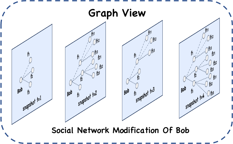
When building a Streaming Graph, a new node and edge can be added to the graph continuously through an incremental data stream, thus dynamically constructing the graph. At the same time, for each incremental data graph construction completion, it can trigger traversal calculation tracking the evolving process of Bob's 2-degree friends over time.

DSL code

set geaflow.dsl.window.size = 1;

CREATE TABLE table_knows (
  personId int,
  friendId int,
  weight int
) WITH (
  type='file',
  geaflow.dsl.file.path = 'resource:///data/table_knows.txt'
);

INSERT INTO social_network.knows
SELECT personId, friendId, weight
FROM table_knows;

CREATE TABLE result (
  personName varchar,
  friendName varchar,
  weight int
) WITH (
	type='console'
);

-- Graph View Name Defined in Graph View Concept --
USE GRAPH social_network;
-- find person id 3's known persons triggered every window.
INSERT INTO result
SELECT
	name,
	known_name,
	weight
FROM (
  MATCH (a:person where a.name = 'Bob') -[e:knows]->{1, 2}(b)
  RETURN a.name as name, b.name as known_name, e.weight as weight
)

HLA code

//build graph view.
final String graphName = "social_network";
GraphViewDesc graphViewDesc = GraphViewBuilder.createGraphView(graphName).build();
pipeline.withView(graphName, graphViewDesc);

// submit pipeLine task.
pipeline.submit(new PipelineTask() {
	@Override
	public void execute(IPipelineTaskContext pipelineTaskCxt) {

        // build vertices streaming source.
		PStreamSource<IVertex<Integer, String>> persons =
			pipelineTaskCxt.buildSource(
				new CollectionSource.(getVertices()), SizeTumblingWindow.of(5000));
		// build edges streaming source.
		PStreamSource<IEdge<Integer, Integer>> knows =
			pipelineTaskCxt.buildSource(
				new CollectionSource<>(getEdges()), SizeTumblingWindow.of(5000));
		// build graphview by graph name.
		PGraphView<Integer, String, Integer> socialNetwork =
			pipelineTaskCxt.buildGraphView(graphName);
		// incremental build graph view.
		PIncGraphView<Integer, String, Integer> incSocialNetwor =
			socialNetwork.appendGraph(vertices, edges);

		// traversal by 'Bob'.
		incGraphView.incrementalTraversal(new IncGraphTraversalAlgorithms(2))
			.start('Bob')
			.map(res -> String.format("%s,%s", res.getResponseId(), res.getResponse()))
			.sink(new ConsoleSink<>());
	}
});