Graph4Stream: Accelerating Stream Computing with Graph-Based Approaches

Author: Kunyu; Reviewer: Dongshuo.

In a previous article "Stream4Graph: Incremental Computation on Dynamic Graphs", we introduced how introducing incremental computation into graph computing—essentially combining "graphs + streams"—allowed Apache GeaFlow (Incubating) to significantly outperform Spark GraphX in terms of performance. Now, the question arises: when we introduce graph computing capabilities into stream computing—combining "streams + graphs"—how does GeaFlow compare to Flink's associative computation performance?

In today’s era, data is being generated at an unprecedented speed and scale, and real-time processing of massive datasets has wide applications in various fields such as anomaly detection, search recommendations, and financial transactions. As one of the core technologies for real-time data processing, stream computing has become increasingly important.

Unlike batch processing, which waits for all data to arrive before computation, stream computing partitions continuously generated data streams into micro-batches and performs incremental computations on each batch. This computational characteristic gives stream computing high throughput and low latency. Common stream computing engines include Flink and Spark Streaming, both of which process data using tabular representations. However, as stream computing applications deepen, more and more scenarios involve computing complex relationships among large datasets, leading to significant performance degradation in table-based stream engines.

Apache GeaFlow (Incubating), an open-source stream graph computing engine, combines graph and stream computing to provide an efficient framework for stream graph processing, significantly improving computational performance. Below, we will introduce the limitations of traditional stream computing engines in relational computation, explain the principles behind GeaFlow's efficiency, and present performance comparisons.

Stream Computing Engine: Flink

Flink is a classic table-based stream processing engine. It slices incoming data streams into micro-batches and processes the data in each batch incrementally. During execution, Flink translates computation tasks into directed graphs composed of basic operators like map, filter, and join. Each operator receives input from upstream and sends output downstream. Incremental data passes through all operators to produce results for the current batch.

Flink Incremental Computation

We take the k-Hop algorithm as an example to illustrate Flink’s computation process. A k-Hop relationship refers to a path that spans k steps—such as a chain of acquaintances in social networks or a sequence of fund transfers in transaction analysis. Assuming a 2-hop relationship, with input data in the format src dst representing pairwise relationships, Flink executes the following SQL:

-- create source table
CREATE TABLE edge (
    src int,
    dst int
) WITH (
);

CREATE VIEW `v_view` (`vid`) AS
SELECT distinct * from
(
SELECT `src` FROM `edge`
UNION ALL
SELECT `dst` FROM `edge`
);

CREATE VIEW `e_view` (`src`, `dst`) AS
SELECT `src`, `dst` FROM `edge`;

CREATE VIEW `join1_edge`(`id1`, `dst`) AS SELECT `v`.`vid`, `e`.`dst`
FROM `v_view` AS `v` INNER JOIN `e_view` AS `e`
ON `v`.`vid` = `e`.`src`;

CREATE VIEW `join1`(`id1`, `id2`) AS SELECT `e`.`id1`, `v`.`vid`
FROM `join1_edge` AS `e` INNER JOIN `v_view` AS `v`
ON `e`.`dst` = `v`.`vid`;

CREATE VIEW `join2_edge`(`id1`, `id2`, `dst`) AS SELECT `v`.`id1`, `v`.`id2`, `e`.`dst`
FROM `join1` AS `v` INNER JOIN `e_view` AS `e`
ON `v`.`id2` = `e`.`src`;

CREATE VIEW `join2`(`id1`, `id2`, `id3`) AS SELECT `e`.`id1`, `e`.`id2`, `v`.`vid`
FROM `join2_edge` AS `e` INNER JOIN `v_view` AS `v`
ON `e`.`dst` = `v`.`vid`;

The execution plan is shown below. It consists of operators such as Aggregate, Calc, and Join. Data flows through each operator to yield incremental results. The core operator, Join, is responsible for relationship lookups. Let's examine how the Join operator works.

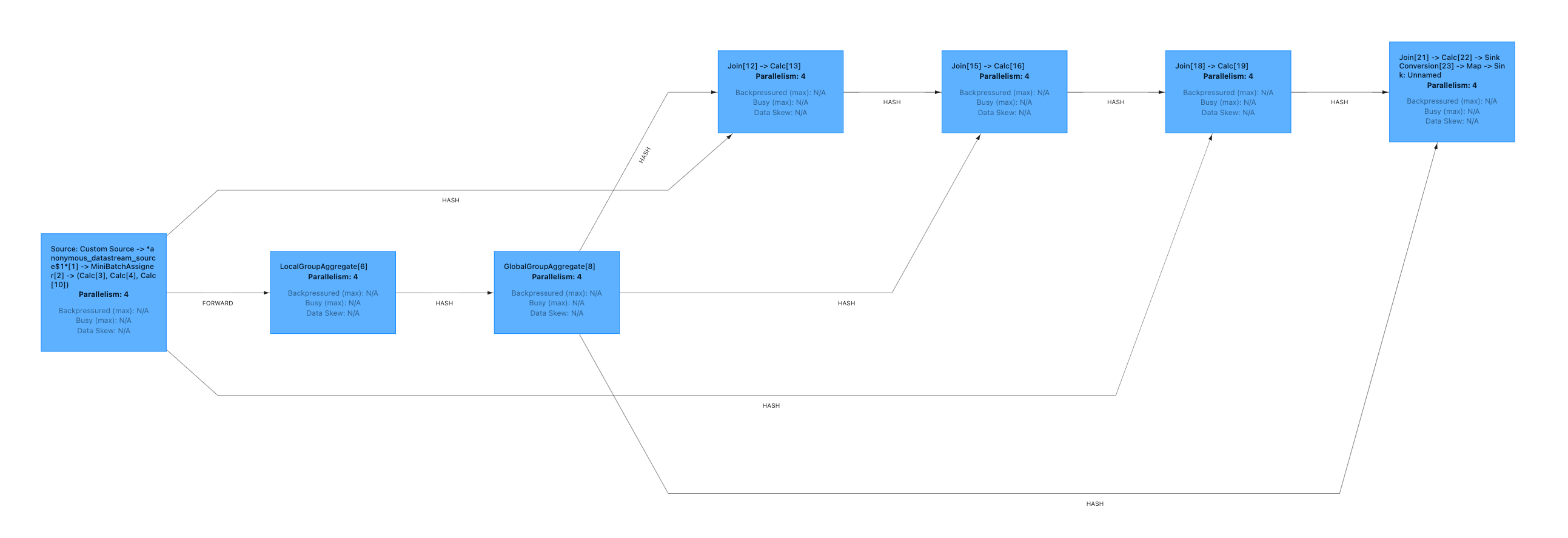
Flink Execution Plan

As shown below, the Join operator has two input streams: LeftInput and RightInput, corresponding to the left and right tables of the join. When data arrives from upstream, the operator begins computation. Taking the left input stream as an example, the data is first stored in LeftStateView. Then, the operator queries RightStateView for data that satisfies the join condition. This querying process requires scanning through RightStateView, and the resulting joined data is passed to the next operator.

The main performance bottleneck lies in scanning RightStateView. LeftStateView and RightStateView store the left and right tables of the join, respectively. As data continuously flows in, the size of StateViews grows, causing scan times to increase dramatically and severely degrading system performance.

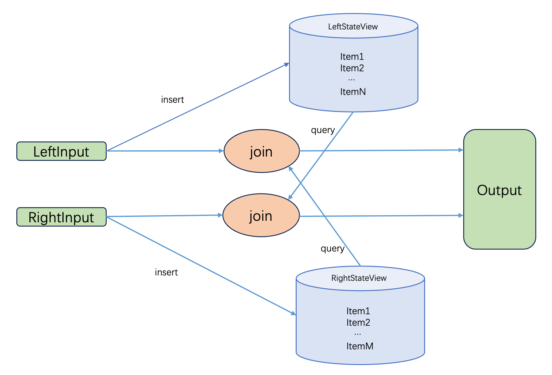
Flink Join Operator Implementation

Stream Graph Computing Engine: Apache GeaFlow (Incubating)

Graph Computing & Stream Graphs

Graph computing is a computational paradigm based on graph data structures. A graph G(V,E) consists of a set of vertices V and edges E, where edges represent relationships between data. Using the public dataset web-Google as an example, each line contains two numbers representing a hyperlink between two web pages. As shown below, the left side shows raw data, which is traditionally modeled as a two-column table. In contrast, graph modeling treats web pages as vertices and hyperlinks as edges, forming a web link graph. In the tabular model, relationship computation is done via joins, which require scanning tables. In graph computing, relationships are directly stored in edges, eliminating the need for scans.

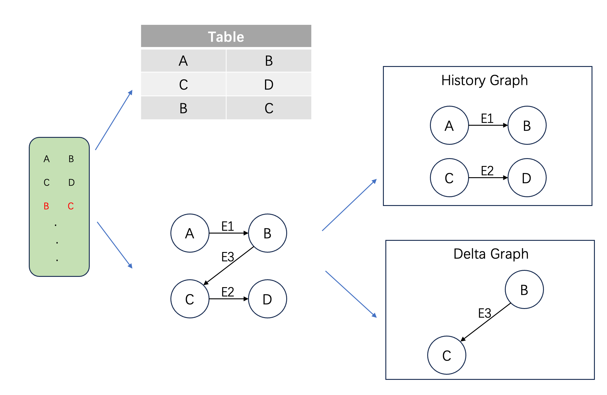
Table Modeling vs. Graph Modeling

A stream graph is the application of graph computing to streaming scenarios. It divides the graph into historical and incremental components based on data stream updates. For example, if the first two rows have been processed and we are now handling the third row, the historical graph is built from the first two rows, and the incremental graph is formed by the third row. Together, they constitute the full graph. Applying incremental graph algorithms on stream graphs enables efficient, real-time computation.

Apache GeaFlow (Incubating) Architecture

The GeaFlow engine’s computation flow consists of stream data input, distributed incremental graph computation, and incremental result output. Like traditional stream engines, real-time data is sliced into micro-batches by window. For each batch, the data is parsed into vertices and edges to form an incremental graph. This incremental graph and the historical graph (built from previous data) together form the complete stream graph. The computation framework applies incremental graph algorithms on the stream graph to yield incremental results, which are then output and added to the historical graph.

Apache GeaFlow (Incubating) Incremental Computation

The GeaFlow computation framework is a vertex-centric iterative model. It starts with vertices in the incremental graph. In each iteration, each vertex maintains its own state and performs computation based on its associated historical and incremental graph data. The result is then passed to neighboring vertices via message passing to trigger the next iteration.

Taking k-Hop as an example, the incremental algorithm works as follows: In the first iteration, all edges in the incremental graph are identified and treated as initial incoming and outgoing paths, which are sent to their start and end vertices. In subsequent iterations, these paths are extended. Once the desired hop count is reached, the paths are sent back to the starting vertex, where they are combined into final results. Detailed implementation can be found in the open-source repository file IncKHopAlgorithm.java.

The diagram below illustrates the two-hop case. In the first iteration, the edge B->C creates incoming and outgoing paths, sent to B and C, respectively. In the second iteration, B receives an incoming path, adds its own incoming edges, and forms a 2-hop incoming path, which it sends to itself. Similarly, C forms a 2-hop outgoing path and sends it to B. In the final iteration, B combines the incoming and outgoing paths to produce the new paths. Unlike Flink, which must scan all historical relationships, GeaFlow's computation is proportional to the incremental paths, not the historical data.

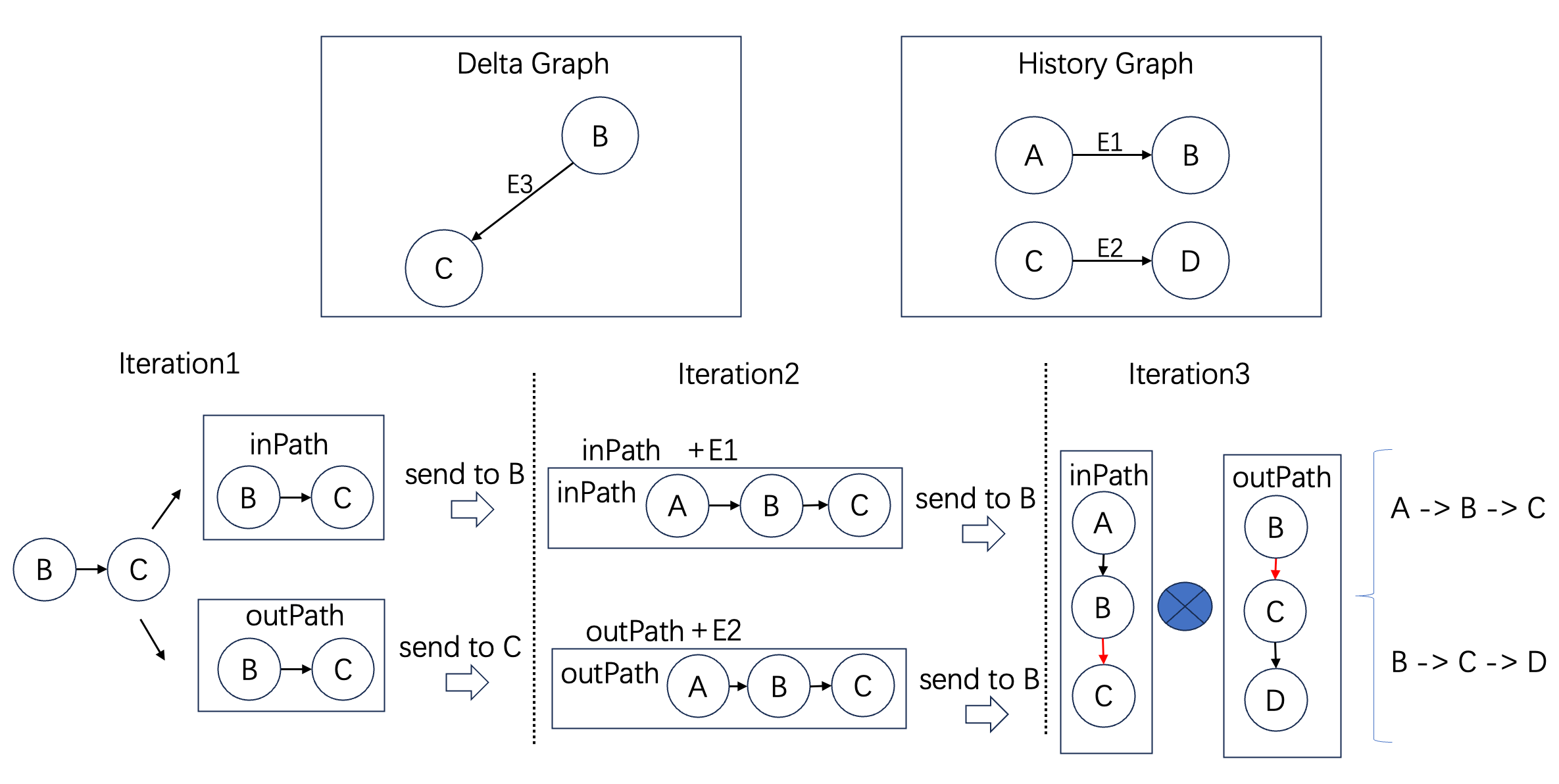
Two-Hop Incremental Path Computation

The above graph algorithm has been integrated into GeaFlow’s IncKHop operator, and users can directly call it using DSL:

set geaflow.dsl.max.traversal=4;
set geaflow.dsl.table.parallelism=4;

CREATE GRAPH modern (
  Vertex node (
    id int ID
  ),
  Edge relation (
    srcId int SOURCE ID,
    targetId int DESTINATION ID
  )
) WITH (
  storeType='rocksdb',
  shardCount = 4
);

CREATE TABLE web_google_20 (
  src varchar,
  dst varchar
) WITH (
  type='file',
  geaflow.dsl.table.parallelism='4',
  geaflow.dsl.column.separator='\t',
  `geaflow.dsl.source.file.parallel.mod`='true',
  geaflow.dsl.file.path = 'resource:///data/web-google-20',
  geaflow.dsl.window.size = 8
);

INSERT INTO modern.node
SELECT cast(src as int)
FROM web_google_20
;

INSERT INTO modern.node
SELECT cast(dst as int)
FROM web_google_20
;

INSERT INTO modern.relation
SELECT cast(src as int), cast(dst as int)
FROM web_google_20;
;

CREATE TABLE tbl_result (
  ret varchar
) WITH (
  type='file',
  geaflow.dsl.file.path='${target}'
);

USE GRAPH modern;

INSERT INTO tbl_result
CALL inc_khop(2) YIELD (ret)
RETURN ret
;

Apache GeaFlow (Incubating) Performance Test

To evaluate GeaFlow’s performance in stream graph computing, we designed a comparative experiment using the k-Hop algorithm. We used the public dataset web-Google.txt as input and measured the time required to complete the computation across one-hop to four-hop scenarios. The experiment ran on 16 servers, each with 8 cores and 16GB memory.

As shown in the results below, the x-axis represents one-hop to four-hop relationships, and the y-axis shows the processing time on a logarithmic scale. In one- and two-hop cases, Flink outperforms GeaFlow due to the small amount of data involved in joins. However, as complexity increases, Flink’s join-based approach becomes inefficient, especially in four-hop cases, where it can’t finish within a day. GeaFlow, by contrast, scales efficiently due to its incremental graph algorithm, whose performance depends only on the incremental paths.

k-Hop Computation Performance Comparison

Conclusion and Future Work

Traditional stream engines like Flink use join operators for relationship computation, which requires scanning all historical data, resulting in poor performance in large-scale associative scenarios. Apache GeaFlow (Incubating) addresses this by introducing graph computing into stream processing through a stream graph framework, significantly boosting performance with incremental graph algorithms.

Apache GeaFlow (Incubating) is now open-source. We aim to build a unified lakehouse engine for graph data to support diverse associative analytics. We are also preparing to join the Apache Software Foundation to enrich the open-source big data ecosystem. If you're interested in graph technology, we welcome you to join the community.

There are many exciting tasks to explore. You can start with these beginner-friendly issues:

• Support incremental k-Core algorithm (Issue 466)
• Support incremental Minimum Spanning Tree algorithm (Issue 465)
• ...

References

1. Apache GeaFlow (Incubating) Project: https://github.com/apache/geaflow
2. web-Google Dataset: https://snap.stanford.edu/data/web-Google.html
3. Apache GeaFlow (Incubating) Issues: https://github.com/apache/geaflow/issues
4. Incremental k-Hop Source Code: https://github.com/apache/geaflow/blob/master/geaflow/geaflow-dsl/geaflow-dsl-plan/src/main/java/com/antgroup/geaflow/dsl/udf/graph/IncKHopAlgorithm.java